HILL Tutorial
Import Data:
The HILL web app reads the 2D class averages as the input. For your own data, you could use the mrc or mrcs file obtained after Class2D in Cryosparc or RELION. HILL supports importing data through upload, url or EMDB ID.
Data Quality Assessment:
After importing the data, we can go through different class averages to assess the quality of the 2D class averages. A good image of a 2D class average should display features of your filament and should not be blurred or noisy. Such images show clear horizontal layer lines in the power spectra plot, and the phase difference plot should show consistently dark blue or yellow layer lines.
There are many factors that contribute to a poor image. For example, if the helical axis is not vertical, slanted layer lines would be observed instead of horizontal layer lines. The helical axis can be adjusted by rotating the image in the app. Below is an example:
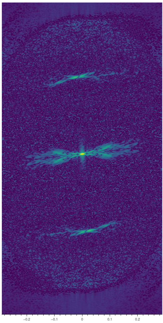
Figure 1
Figure 1 above shows a case where the layer lines are slanted. If this is the case, you can adjust the rotation of the image by the image parameters toolbox below the original image (Figure 2) until the layer lines get horizontal:
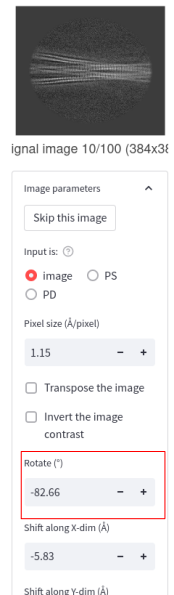
Figure 2
Another factor that affects the layer line indexing is the out-of-plane tilt of the filaments. In ideal conditions of grid preparation and uniform ice thickness, filaments are expected to be perpendicular to the electron beam. However, in practice, some grids can be bent or undulated or have non-uniform ice thickness. Hence the filaments are not exactly perpendicular to the beam and may have an out of plane tilt. Presence of out-of-plane tilt would complicate helical indexing and thus you should avoid images with large out-of-plane tilts. The phase difference (PD) across the meridian plot can be used as a sensitive gauge of the out-of-plane tilt angle: the PD plot of an image with out-of-plane tilt will show layer lines with a mosaic of blue and yellow (Figure 3) and you should avoid using those images for indexing. Instead, focus on images that give dark blue or bright yellow layer lines in the PD plot
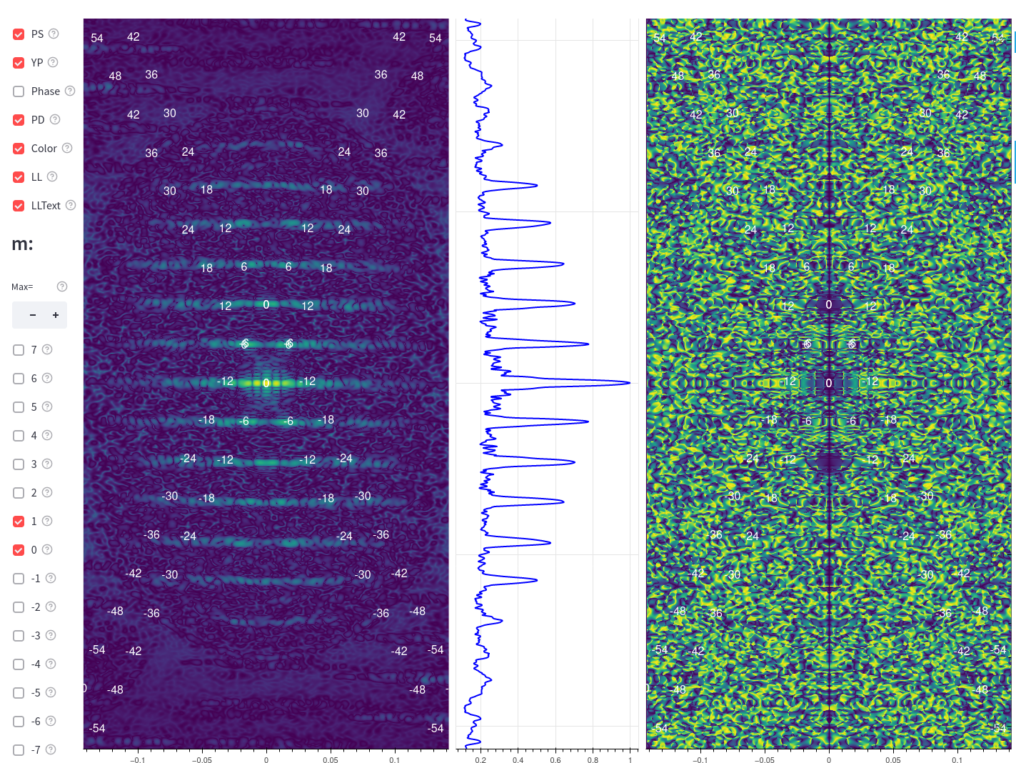
Figure 3
After selecting a good 2D class image or the 3D projection with the minimum out-of-plane tilt displaying clear layer lines in both the power spectra and PD plots, we begin to index the power spectra/helical diffraction.
Helical assemblies can have additional rotational symmetry such as two-fold, three-fold, four-fold, and so on. In sections below, we will see one example with odd rotational -symmetry and another with even rotational-symmetry.
Example 1: VipA/VipB
Example Data:
In the selection box, select url. Input the url link below:
Then choose the 2nd image out of the 13 images.
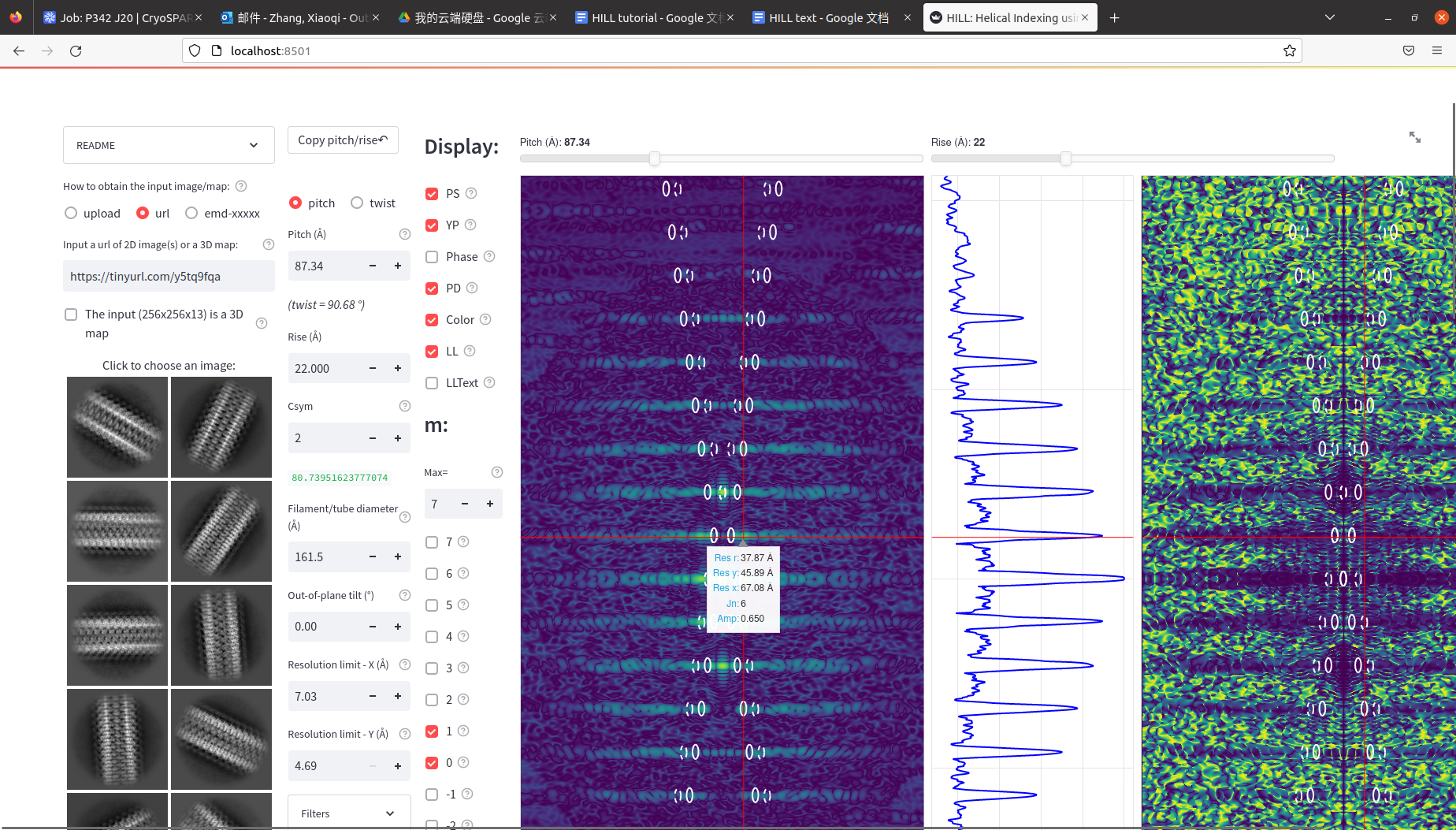
Looking at the power spectra and the PD plot (Figure 4), we can see clear horizontal layer lines and the corresponding dark blue region in the PD plot. By default, the program will display two X patterns of layer lines with m=0 and m=1, with numeric labels of the Bessel orders corresponding to each layer line. By unchecking the LLtext selection box, the position of the layer lines would be shown as ellipses.
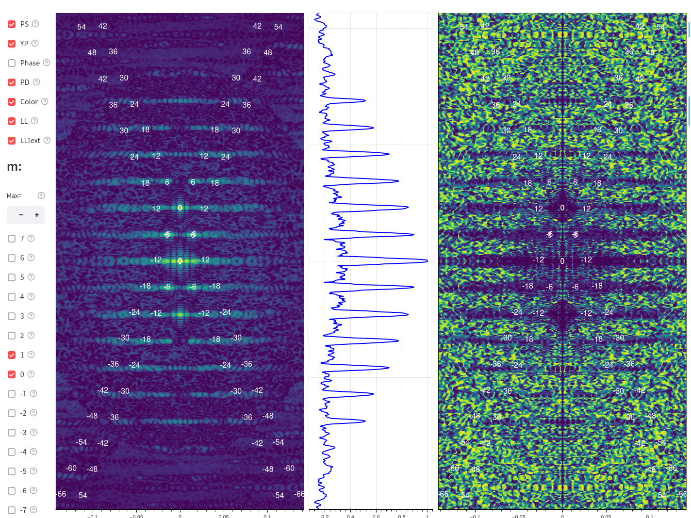
Figure 4
After importing the input, you can see an image of the projection of the helix. When hovering the mouse on the image of the helix, a hover tip box will show the coordinate in Å corresponding to the position of the cursor. Below the transformed image, you can also see a radial profile plot showing the distribution of the density along the radius (Figure 5). You will notice on the left of the power spectra plot that the diameter of the filament is a parameter needed for helical indexing. The diameter here is used for the estimation of the Bessel order of the layer lines. Usually, it’s not recommended to use the diameter estimated by measuring at the edge of the filament or simply using the peak in the radial profile plot. The HILL app will provide you by default with an estimation of the filament diameter, based on a core-shell two layer cylinder model and estimating its center of mass along the radius. We suggest using the default estimated diameter for indexing unless there is some confusion with the estimation of the Bessel orders.
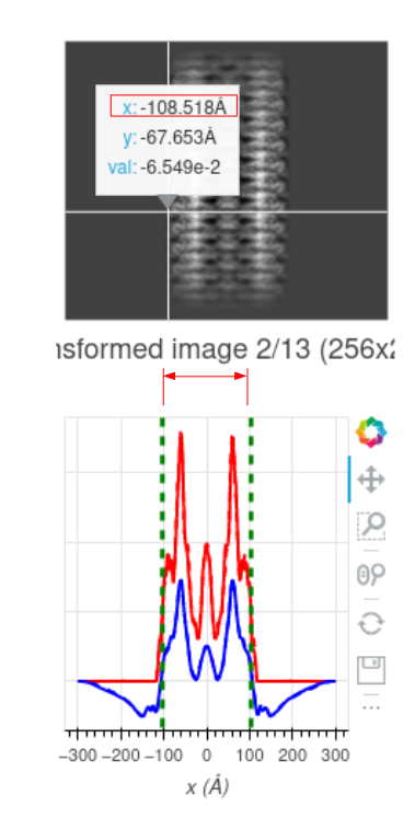
Figure 5
Before we start, another useful tip is to adjust the resolution limit on the X and Y axis. By setting the resolution limit to lower resolutions, we will be able to focus more on the region closer to the center of the power spectra and phase difference plot.
Estimation of the helical rise:
In this example, a precise estimate of the helical rise is obtained by changing the Rise slider to match the center of X patterns (m = 1 or -1) with the peaks on the meridian in the power spectrum plot (Figure 6).
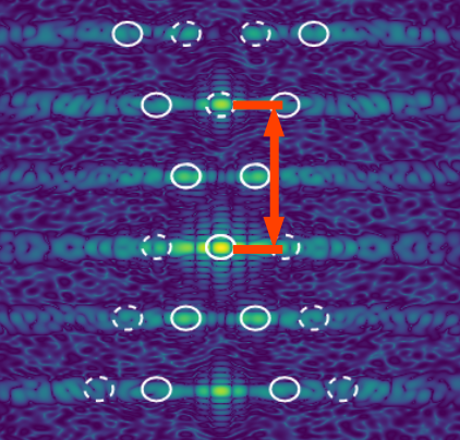
Figure 6
Effectively, increasing the rise will decrease the distance between the center of the X patterns (labeled in red in Figure 6)
Note that the peak in the power spectra plot on the meridian does not always correspond to the rise. Sometimes, out-of-plane tilt could also result in artificial peaks on the meridian, so it’s important to assess the out-of-plane tilt by looking at the phase difference plot before we start the helical indexing.
Estimation of the helical pitch and c-symmetry:
After we get the rise, we can fix the rise and adjust the pitch and c-symmetry.
We can adjust the pitch by dragging the Pitch slider above the power spectra plot. Effectively, increasing the helical pitch would decrease the distance along the meridian between the labeled layerlines (Figure 7):
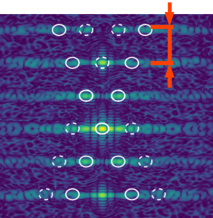
Figure 7
For the c-symmetry, we should first look at the phase difference plot. If the phase difference along the layer line shows consistent blue regions (PD = 0 degree), it means the Bessel order of the layer lines should be even, which is the case of this example. That means we should only try even c-symmetry orders (2, 4, 6, 8, …) If there are phase differences along the layer lines that show consistent yellow regions (PD = 180 degree), it means the Bessel order of those layer lines is odd (1, 3, 5, …). We will see an example of that in the next section.
Starting with a C2 symmetry, our goal is to match the adjacent ellipses (which correspond to layer lines with Bessel order difference of 2, where 2 is the current c-symmetry order we are setting) with the peaks in the power spectra.
After adjusting the pitch, we should look at whether the labeled first peaks (the ellipses) overlap with the first peak of the layer lines in the power spectra. If we hover the cursor on the first peak in the power spectra, we will see in the hover tip the estimated Bessel order of this layer line (Jn), assuming the cursor position is the first peak.
We might find a range of Bessel orders suitable if we move around the region that we think is a peak (for example, 4, 5, 6). In this case, the PD plot can be useful to determine whether the Bessel order of the layer line is even or odd. We can adjust the c-symmetry to fit the ellipse with the first peak of the layer line in the power spectra.
The first peak off the meridian of each layer line in the power spectra should correspond with the first peak of the Bessel function. The distance (\(r\)) from the meridian to the first peak of the Bessel function \(J_{n}(2\pi Rr)\) in the power spectra is determined by the Bessel order (\(n\)) and the diameter of the filament (\(R\)) in real space. The peak position \(X_{0}\) of a specific Bessel function is determined by its Bessel order \(n\) (a common approximation is \(X_{0} = n + 2\)), thus \(X_{0} = 2\pi Rr\) is fixed. Therefore, the position of the first peak in the power spectra (determined by \(r\)) is determined by the Bessel order, and inverse proportional to the filament diameter in real space.
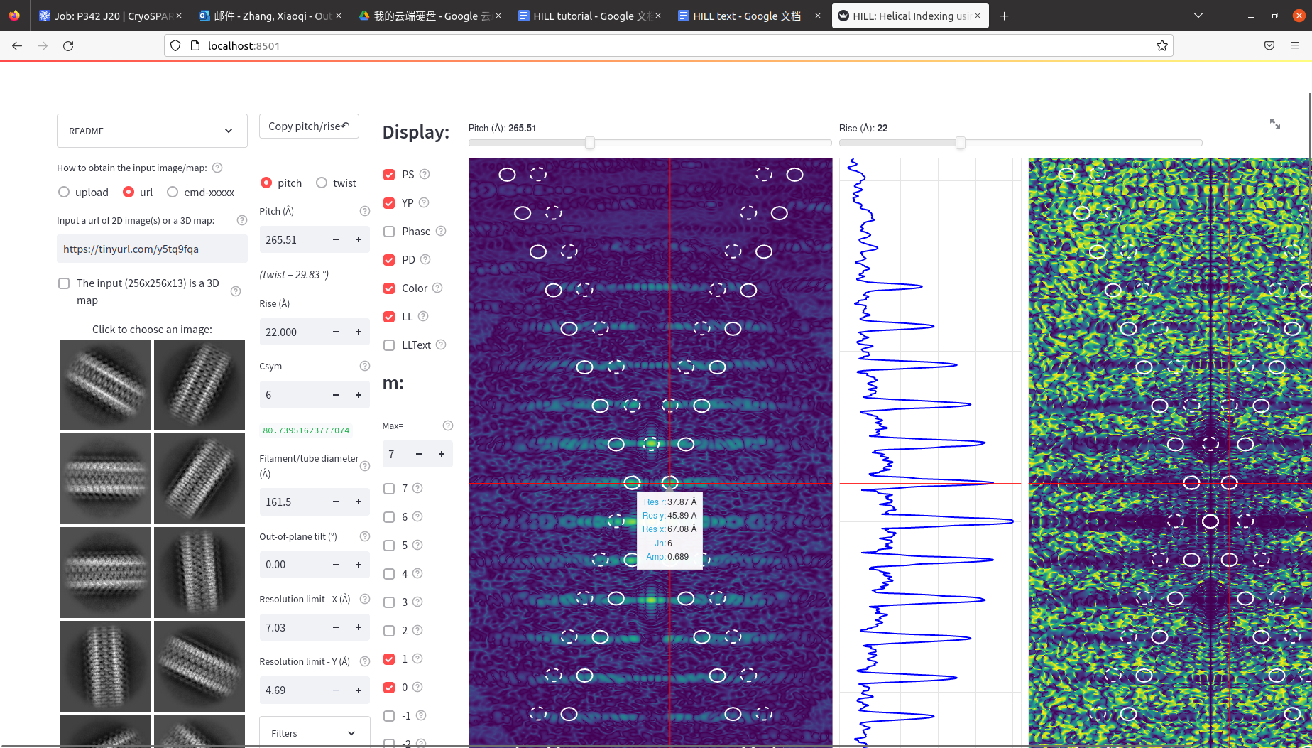
Here in this case, we can find that the peak best matches with the ellipses when Csym=6, after adjusting the pitch when we change the c-symmetry. Now, we have a good estimation of the parameters. After this, we can record the rise, pitch/twist and the c-symmetry parameters and move on.
Example 2: EMD-26987 F-Actin
Select the 3rd input option “emd-xxxxx” and Input the EMDB ID: emd-26987. With the images and the helical parameters reported in the EMDB entry, the plots are below (Figure 13):
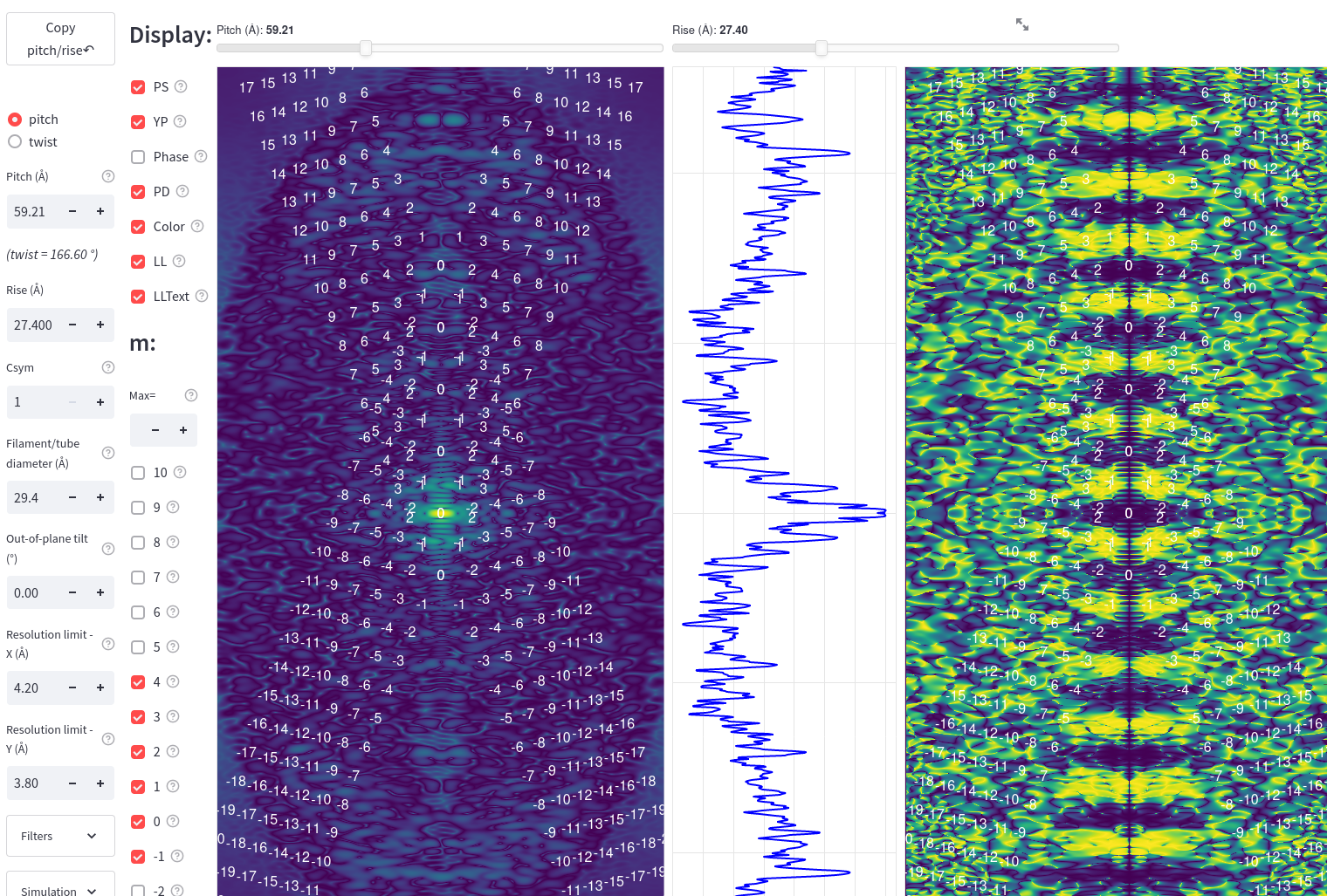
Figure 13
We can see in the phase difference plot there are alternating blue and yellow layer lines, indicating an odd c-symmetry order. If only looking at the power spectra plot, it might be hard to align the labeled layer lines with the peaks in the power spectra plot. However, in this case, we can see the phase difference plot shows clear separation of blue and yellow layer lines. With the reported helical parameters, we can see that the labeled layer line peaks with even bessel orders fall into the blue regions in the PD plot, and the ones with odd bessel orders fall into the yellow regions in the PD plot. We can also see the centers of the X patterns fall into the center of the blue regions on the meridian. This would be an example of what it would look like when the c-symmetry is odd, and that the clear patterns in the PD plot can be helpful for determining the helical parameters when the power spectra is not very clear to interpret.
Example 3: EMD-10129 TMV
Select the 3rd input option “emd-xxxxx” and Input the EMDB ID: emd-10129. With the images and the helical parameters reported in the EMDB entry, the plots are below (Figure 14):
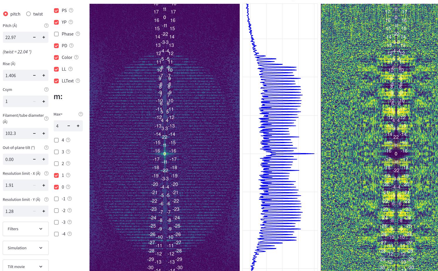
Figure 14
We can see very many layer lines in this example. Notice from the reported helical parameter, the helix has a very small rise value, which results in a very large distance between the center of the X patterns. From the plot we can see that the center of the X pattern cannot be matched with any layer lines we can observe in the plot. In this case, we cannot first determine the helical rise. Instead, we need to match the layer lines from the many far away X patterns with the peaks based on the bessel order of the layer lines and the phase difference pattern in the PD plot. By adjusting the X/Y resolution limit to 5 Angstrom, we can see the zoomed-in plots below (Figure 15):
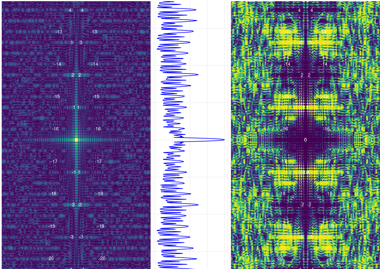
Figure 15
Example 4: PHF Tau
In the selection box, select url. Input the url link below:
(link)
This is an example of a 2D class average image that ensembles the characteristics of PHF tau from our own processing of the dataset EMPIAR-10230 using RELION. With these helical parameters: rise=2.375, pitch=4.75, the plots are below (Figure 16):
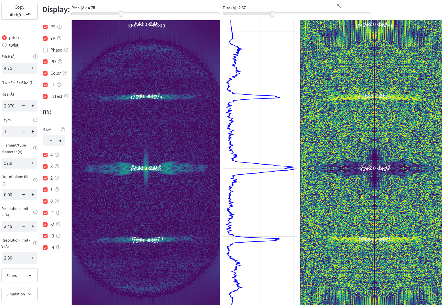
Figure 16
In the case of PHF tau, it is reported to have a 2-sub-1 symmetry, which is practically a type of C1 symmetry, with the rise of 2.375 Angstrom (which is a half of the rise of normal amyloids 4.75 Angstrom) and a twist of 179.45 degree. These parameters will lead to a very large distance between the centers of the X patterns, and a very small pitch of 4.75 Angstrom. This will result in a very small distance between the adjacent layer lines. From the plot, we can see that layer lines from multiple X patterns far away from the equator with an odd bessel order and those with an even layer line respectively form the 3 peak regions in the power spectra. We are expecting to see the phase difference plot at the equator to show consistently blue and those other two regions to show consistently yellow.
Example 5: EMD-0260 SF Tau
Select the 3rd input option “emd-xxxxx” and Input the EMDB ID: emd-0260. With the images and the helical parameters reported in the EMDB entry, the plots are below (Figure 18):
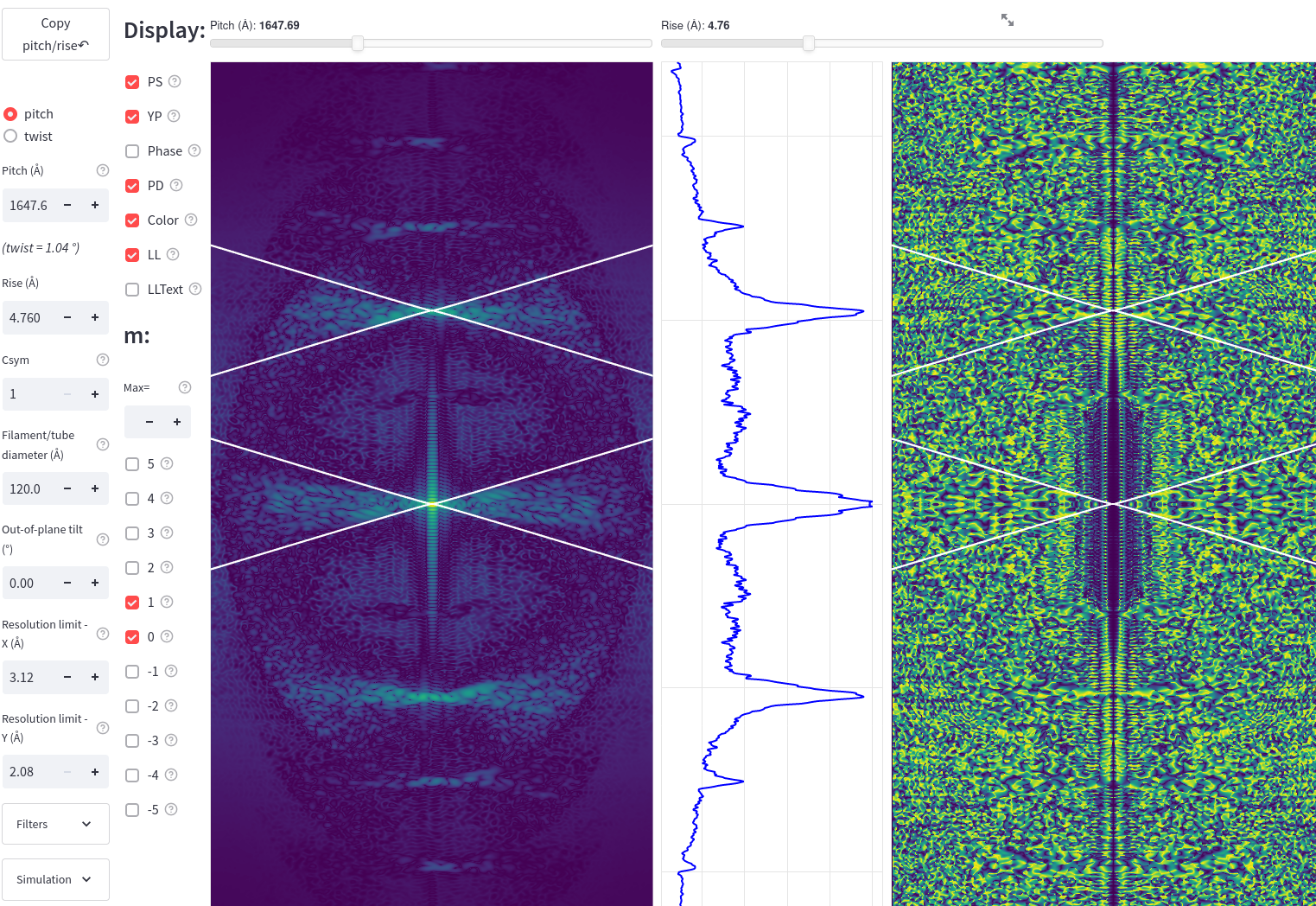
Figure 18
In this example, we are able to match the center of the X patterns with the peaks in the power spectra plot with the rise around 4.75. The reported helical parameters indicate that the filament has a very large pitch. This will result in the small distance between the adjacent layer lines. As a result, the X patterns can be very flat with dense layer lines. One feature we can use to distinguish between the SF tau and the PHF tau would be the difference in the PD pattern. In the PHF tau we saw in the previous example, the PD of layer lines off the equators (for example m = 1 or -1) will show consistent yellow. Here for SF tau, with the c-symmetry of 1, the layer line with a Bessel order of 0 would be located at the meridian, so we can see the peak at the meridian corresponding with the blue region in the PD plot (Figure 19).
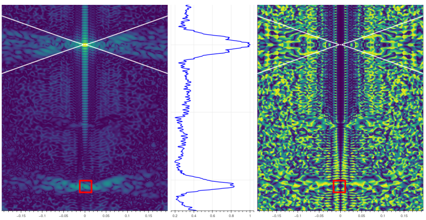
Figure 19
The PD of the remaining adjacent layer lines with alternating odd and even bessel orders will show adjacent blue and yellow. Below is another example of a 2D class average image that ensembles such characteristics of SF tau from our own processing of the dataset EMPIAR-10230 using RELION (Figure 20, Figure 21):
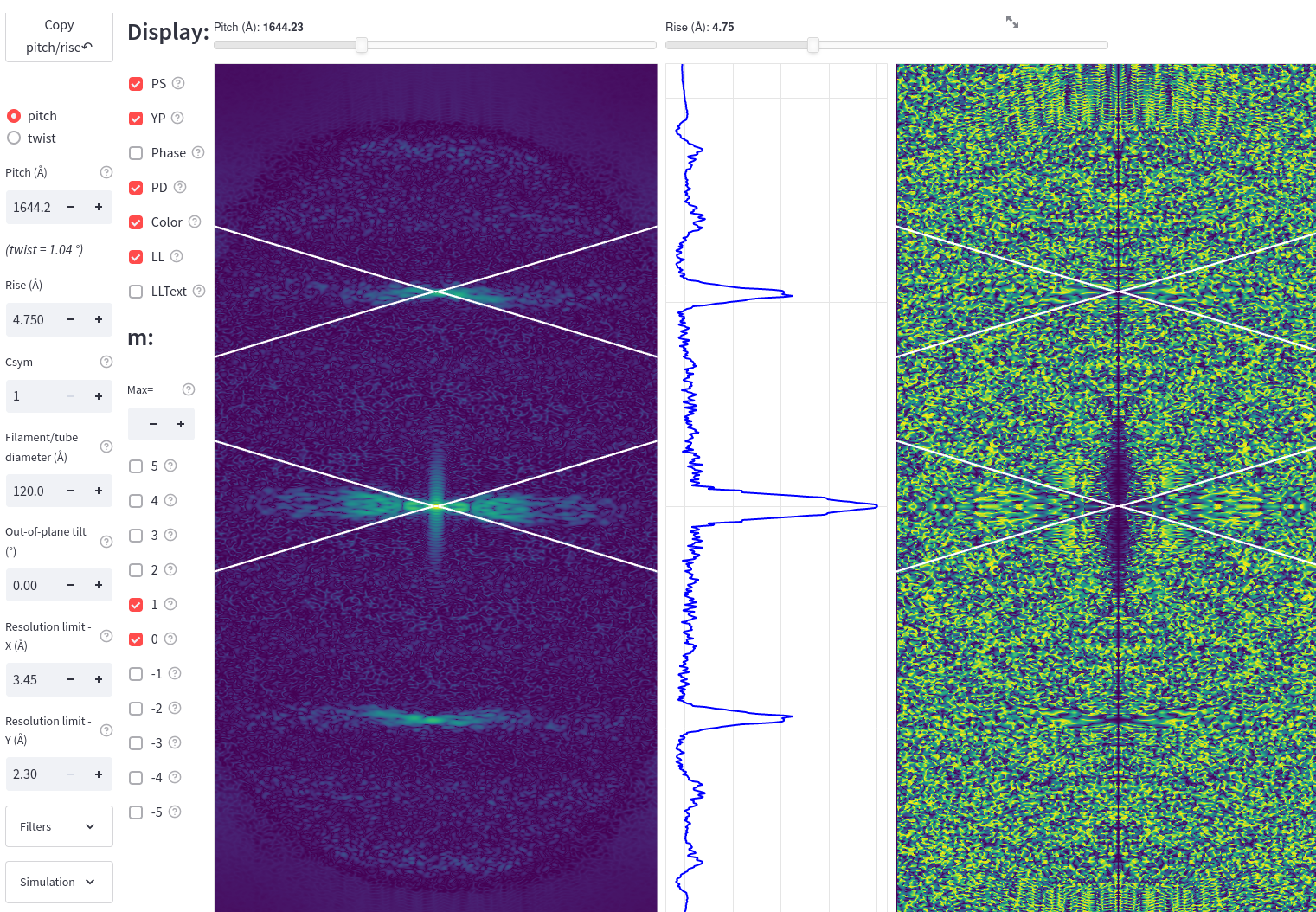
Figure 20
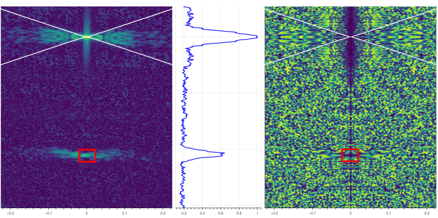
Figure 21